Recognizing Human Emotions is a complex task and it not only requires the understanding of the words or the sentences but also facial expressions, body languages, tone of the speaker, etc.
That is why to correctly understand what the speaker is trying to convey or to understand their emotions it is preferred to have in-person talks rather than phone calls and phone calls are preferred over texts and messages.
In today’s world we all are well aware of the Voice Recognition AI Models or Voice Command AI Model, but AI is not just limited to that.
Have you ever thought that it would be wonderful to have an AI model to understand your emotions when you give commands to it or talk to it and behave accordingly, or when listening to songs on your favorite app the AI model should recognize your emotion and suggest you songs accordingly. Wouldn’t be amazing?
That’s what Speech Emotion Recognition does. On the basis of your speech it detects your emotion. In this article we will be talking about one such Deep Learning Model.
Introduction to cAInvas
cAInvas is an integrated development platform to create intelligent edge devices. Not only we can train our deep learning model using Tensorflow, Keras, or Pytorch we can also compile our model with its edge compiler called DeepC to deploy our working model on edge devices for production. The Heartbeat Anomaly Detection model which we are going to talk about, was developed in cAInvas.
Why cAInvas
cAInvas is an ideal choice to develop Deep Learning models because of the simplicity it provides to develop even the most complex Deep Learning Models and also because of an amazing UseCase Gallery which contains pre-written codes for the development of various Deep Learning Models. Our Speech Emotion Recognition is also part of the cAInvas’ gallery.
Source of Data
While working in cAInvas one of its key features is UseCases Gallary. When working on any of its UseCases you don’t have to look for data manually.
As they have the feature to import your dataset to your workspace when you work on them. To load the data we just have to enter the following commands:
Exploratory Data Analysis

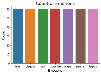
In this step we gain intuition about the dataset provided and as we can see that we have a balanced dataset and the emotions which we will be detecting are: Fear, Disgust, Sad, Surprise, Angry, Neutral and Happy.
The dataset contains audio data and we can plot waveplots and spectograms for audio signals to understand our Data.
- Waveplots — Waveplots let us know the loudness of the audio at a given time.
- Spectograms — A spectrogram is a visual representation of the spectrum of frequencies of sound or other signals as they vary with time. It’s a representation of frequencies changing with respect to time for given audio/music signals.
This can be done by implementing the following function.
We also perform data augmentation to our data such as introduction of some noise, stretching the audio signals, perform some shift in the audio signals and also perform some augmentations in the pitch of the audio signals. This augmentation will help us to produce better training results.
Feature Extraction
Extraction of features is a very important part in analyzing and finding relations between different things. As we already know that the data provided of audio cannot be understood by the models directly so we need to convert them into an understandable format for which feature extraction is used.
In this project we are not going to extracting 5 audio features:
- Zero Crossing Rate
- Chroma_stft
- MFCC
- RMS(root mean square) value
- MelSpectogram to train our model.
And once the data is prepared we will begin our training process.
Model Training
After feature extraction next step is to pass our extracted feature as training data for our Deep Learning model along with the target labels so that our model can learn to classify Emotions on the basis of speech sound.
The model architecture used was:
Model: "sequential"
_________________________________________________________________
Layer (type)                 Output Shape              Param #
=================================================================
conv1d (Conv1D)              (None, 162, 256)          2304
_________________________________________________________________
conv1d_1 (Conv1D)            (None, 162, 256)          524544
_________________________________________________________________
batch_normalization (BatchNo (None, 162, 256)          1024
_________________________________________________________________
dropout (Dropout)            (None, 162, 256)          0
_________________________________________________________________
max_pooling1d (MaxPooling1D) (None, 20, 256)           0
_________________________________________________________________
conv1d_2 (Conv1D)            (None, 20, 128)           262272
_________________________________________________________________
conv1d_3 (Conv1D)            (None, 20, 128)           131200
_________________________________________________________________
dropout_1 (Dropout)          (None, 20, 128)           0
_________________________________________________________________
conv1d_4 (Conv1D)            (None, 20, 128)           131200
_________________________________________________________________
conv1d_5 (Conv1D)            (None, 20, 128)           131200
_________________________________________________________________
batch_normalization_1 (Batch (None, 20, 128)           512
_________________________________________________________________
dropout_2 (Dropout)          (None, 20, 128)           0
_________________________________________________________________
max_pooling1d_1 (MaxPooling1 (None, 2, 128)            0
_________________________________________________________________
conv1d_6 (Conv1D)            (None, 2, 64)             65600
_________________________________________________________________
conv1d_7 (Conv1D)            (None, 2, 64)             32832
_________________________________________________________________
flatten (Flatten)            (None, 128)               0
_________________________________________________________________
dense (Dense)                (None, 7)                 903
=================================================================
Total params: 1,283,591
Trainable params: 1,282,823
Non-trainable params: 768
_________________________________________________________________
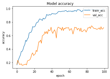
The loss function used was “categorical_crossentropy” and optimizer used was “Adam”.For training the model we used Keras API with tensorflow at backend. The model showed good performance achieving a decent accuracy. Here is the accuracy curve for the model:

Also Read: Recognise Arabic Digits
Introduction to DeepC
DeepC Compiler and inference framework is designed to enable and perform deep learning neural networks by focussing on features of small form-factor devices like micro-controllers, eFPGAs, cpus, and other embedded devices like raspberry-pi, odroid, Arduino, SparkFun Edge, risc-V, mobile phones, x86 and arm laptops among others.
DeepC also offers ahead of time compiler producing optimized executable based on LLVM compiler tool chain specialized for deep neural networks with ONNX as front end.
Compilation with DeepC
After training the model, it was saved in an H5 format using Keras as it easily stores the weights and model configuration in a single file. For this, we used Keras checkpoints and save only the best model.
After saving the file in H5 format we can easily compile our model using DeepC compiler which comes as a part of cAInvas platform so that it converts our saved model to a format which can be easily deployed to edge devices. And all this can be done very easily using a simple command.
And our model is ready for deployment.👍
Link for the cAInvas Notebook: https://cainvas.ai-tech.systems/use-cases/speech-emotion-recognition-app/
Credit: Ashish Arya
