A Mineral Classifier can be used to identify the minerals just by looking at their photographs without any need of human intervention and can thus help humans in mineral exploration. It can help metals and mining industry speed up the mineral identification process and will also help in finding the new drill targets.

Table of Content

• Introduction to cAInvas
• Source of Data
• Data Visualization and Analysis
• Trainset-TestSet Creation
• Model Training
• Introduction to DeepC
• Compilation with DeepC

Introduction to cAInvas

cAInvas is an integrated development platform to create intelligent edge devices. Not only we can train our deep learning model using Tensorflow, Keras or Pytorch, we can also compile our model with its edge compiler called DeepC to deploy our working model on edge devices for production.

The Mineral Classification model which we are going to talk about, is also developed on cAInvas. All the dependencies which you will be needing for this project are also pre-installed.

cAInvas also offers various other deep learning notebooks in its gallery which one can use for reference or to gain insight about deep learning. It also has GPU support and which makes it the best in its kind.

Source of Data

While working on cAInvas one of its key features is UseCases Gallary. When working on any of its UseCases you don’t have to look for data manually. As they have the feature to import the dataset to your workspace when you work on them. To load the data we just have to enter the following commands:

Running the above command will load the labelled data in your workspace which you will use for model training.

Data Visualization and Data Analysis

Next step in the pipeline is to visualize and analyze our data so as to gain intuition about data and what we are dealing with. For this we printed out first 20 samples of data from dataset which consisted of seven different classes of images. For this we ran the following command:

Next we checked for any class imbalance in our data. So we plotted a bar graph. The bar graph is shown below:

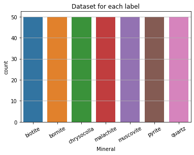
As we can see that the data set is balanced. Next we obtained the maximum height and width of the image and mean height and width of the images present in our dataset. For this we ran the following command:

TrainSet-TestSet Creation

Next we will create the train and test dataset for training our deep learning model. For this we will use ImageDataGenerator Module of the Keras Image Preprocessing Library. This will load the images along with their labels for us in a format which is recognizable by Keras for further training process.

We simply have to create the train_generator and test_generator and then when we run them they will create the dataset for us. The following commands will give you an idea on how to create the train dataset and then you will be able to create the testset on your own.

Model Training

After creating the dataset next step is to pass our training data for our Deep Learning model to learn to identify or classify different classes of images. The model architecture used was:

Model: "model"
_________________________________________________________________
Layer (type)                 Output Shape              Param #   
=================================================================
input_1 (InputLayer)         [(None, 224, 224, 3)]     0         
_________________________________________________________________
block1_conv1 (Conv2D)        (None, 224, 224, 64)      1792      
_________________________________________________________________
block1_conv2 (Conv2D)        (None, 224, 224, 64)      36928     
_________________________________________________________________
block1_pool (MaxPooling2D)   (None, 112, 112, 64)      0         
_________________________________________________________________
block2_conv1 (Conv2D)        (None, 112, 112, 128)     73856     
_________________________________________________________________
block2_conv2 (Conv2D)        (None, 112, 112, 128)     147584    
_________________________________________________________________
block2_pool (MaxPooling2D)   (None, 56, 56, 128)       0         
_________________________________________________________________
block3_conv1 (Conv2D)        (None, 56, 56, 256)       295168    
_________________________________________________________________
block3_conv2 (Conv2D)        (None, 56, 56, 256)       590080    
_________________________________________________________________
block3_conv3 (Conv2D)        (None, 56, 56, 256)       590080    
_________________________________________________________________
block3_pool (MaxPooling2D)   (None, 28, 28, 256)       0         
_________________________________________________________________
block4_conv1 (Conv2D)        (None, 28, 28, 512)       1180160   
_________________________________________________________________
block4_conv2 (Conv2D)        (None, 28, 28, 512)       2359808   
_________________________________________________________________
block4_conv3 (Conv2D)        (None, 28, 28, 512)       2359808   
_________________________________________________________________
block4_pool (MaxPooling2D)   (None, 14, 14, 512)       0         
_________________________________________________________________
block5_conv1 (Conv2D)        (None, 14, 14, 512)       2359808   
_________________________________________________________________
block5_conv2 (Conv2D)        (None, 14, 14, 512)       2359808   
_________________________________________________________________
block5_conv3 (Conv2D)        (None, 14, 14, 512)       2359808   
_________________________________________________________________
block5_pool (MaxPooling2D)   (None, 7, 7, 512)         0         
_________________________________________________________________
average_pooling2d (AveragePo (None, 3, 3, 512)         0         
_________________________________________________________________
flatten (Flatten)            (None, 4608)              0         
_________________________________________________________________
dense (Dense)                (None, 128)               589952    
_________________________________________________________________
dropout (Dropout)            (None, 128)               0         
_________________________________________________________________
dense_1 (Dense)              (None, 7)                 903       
=================================================================
Total params: 15,305,543
Trainable params: 590,855
Non-trainable params: 14,714,688
_________________________________________________________________

We have used a VGG-16 pretrained model and have applied transfer learning. We have modified the last dense layer of the VGG model according to our needs. We will not train the entire VGG model but only certain layers which we have added to our pre-existing model.

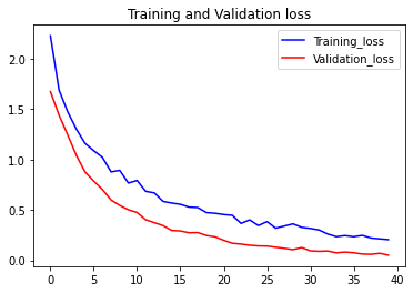
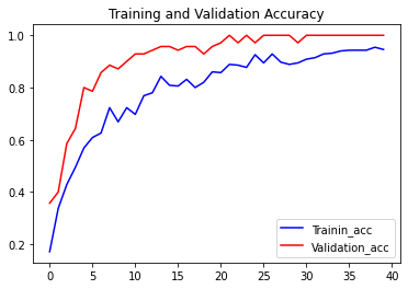
The loss function used was “categorical_crossentropy” and optimizer used was “Adam”.For training the model we used Keras API with tensorflow at backend. The model showed good performance achieving a decent accuracy. Here are the training plots for the model:

Introduction to DeepC

DeepC Compiler and inference framework is designed to enable and perform deep learning neural networks by focussing on features of small form-factor devices like micro-controllers, eFPGAs, cpus and other embedded devices like raspberry-pi, odroid, arduino, SparkFun Edge, risc-V, mobile phones, x86 and arm laptops among others.

DeepC also offers ahead of time compiler producing optimized executable based on LLVM compiler tool chain specialized for deep neural networks with ONNX as front end.

Compilation with DeepC

After training the model, it was saved in an H5 format using Keras as it easily stores the weights and model configuration in a single file.

After saving the file in H5 format we can easily compile our model using DeepC compiler which comes as a part of cAInvas platform so that it converts our saved model to a format which can be easily deployed to edge devices. And all this can be done very easily using a simple command.

And that’s it, it is that easy to create a mineral classification model which is also ready for deployment on edge devices.

Link for the cAInvas Notebook: https://cainvas.ai-tech.systems/use-cases/mineral-classification-app/

Credit: Ashish Arya