
In this article, we will focus on building a Convolutional Neural Network (CNN), to recognize and classify images from The CIFAR-10 dataset.
The CIFAR-10 dataset is a standard dataset used in computer vision and deep learning community. It consists of 60000 32×32 color images in 10 classes, with 6000 images per class. There are 50000 training images and 10000 test images.
In this tutorial, we will build a convolutional neural network model from scratch using TensorFlow, train that model, and then evaluate its performance on unseen data.
Let’s get started now!
The dataset is split into training and testing sets. The training set consists of 50000 images, with 5000 images of each class, and the testing set consists of 10000 images, with 1000 images from each class.
Loading the dataset
| # Import the CIFAR-10 dataset from keras' datasets | |
| from tensorflow.keras.datasets import cifar10 | |
| # Import this PyPlot to visualize images | |
| import matplotlib.pyplot as plt | |
| %matplotlib inline | |
| import numpy as np | |
| from sklearn.utils import shuffle | |
| # Load dataset | |
| (X_train, Y_train), (X_test, Y_test) = cifar10.load_data() |
- X_train has 50000 training images, each 32 pixels wide, 32 pixels high, and 3 color channels
- X_test has 10000 testing images, each 32 pixels wide, 32 pixels high, and 3 color channels
- Y_train has 50000 labels
- Y_test has 10000 labels.
Now, let’s look at some random images from the training set. You can change the number of columns and rows to get more/less images.
| # show random images from training set | |
| cols = 8 # Number of columns | |
| rows = 4 # Number of rows | |
| fig = plt.figure(figsize=(2 * cols, 2 * rows)) | |
| # Add subplot for each random image | |
| for col in range(cols): | |
| for row in range(rows): | |
| random_index = np.random.randint(0, len(Y_train)) # Pick a random index for sampling the image | |
| ax = fig.add_subplot(rows, cols, col * rows + row + 1) # Add a sub-plot at (row, col) | |
| ax.grid(b=False) # Get rid of the grids | |
| ax.axis("off") # Get rid of the axis | |
| ax.imshow(X_train[random_index, :]) # Show random image | |
| ax.set_title(CIFAR10_CLASSES[Y_train[random_index][0]]) # Set title of the sub-plot | |
| plt.show() # Show the image |
Prepare Training and Testing Data
Before defining the model and training the model, let us prepare the training and testing data. We will use TensorFlow’s version 2.2.0 and Keras’ version 2.3.0-tf for this project. Adding on to this, we will also normalize the inputs, to train the model faster and prevent exploding gradients. Finally, we have to convert the labels to one-hot coded vectors.
| import tensorflow as tf | |
| import numpy as np | |
| print("TensorFlow's version is", tf.__version__) | |
| print("Keras' version is", tf.keras.__version__) | |
| # Normalize training and testing pixel values | |
| X_train_normalized = X_train / 255 - 0.5 | |
| X_test_normalized = X_test / 255 - 0.5 | |
| # Convert class vectors to binary class matrices. | |
| Y_train_coded = tf.keras.utils.to_categorical(Y_train, NUM_CLASSES) | |
| Y_test_coded = tf.keras.utils.to_categorical(Y_test, NUM_CLASSES) |
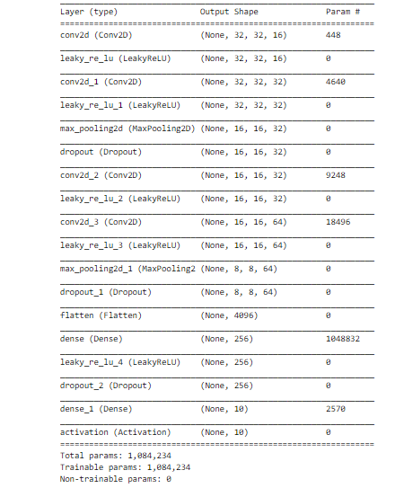
Design your Convolutional Neural Network (CNN)
In our CNN, we have the following layers with certain specifications:
- Convolutional layer which takes (32, 32, 3) shaped images as input, outputs 16 filters, and has a kernel size of (3, 3), with the same padding, and uses LeakyReLU as activation function
- Convolutional layer which takes (32, 32, 16) shaped tensor as input, outputs 32 filters, and has a kernel size of (3, 3), with the same padding, and uses LeakyReLU as activation function
- Max Pool layer with pool size of (2, 2), this outputs (16, 16, 16) tensor
- Dropout layer with the dropout rate of 0.25, to prevent overfitting
- Convolutional layer which takes (16, 16, 16) shaped tensor as input, outputs 32 filters, and has a kernel size of (3, 3), with the same padding, and uses LeakyReLU as activation function
- Convolutional layer which takes (16, 16, 32) shaped tensor as input, outputs 64 filters, and has a kernel size of (3, 3), with the same padding, and uses LeakyReLU as activation function
- Max Pool layer with pool size of (2, 2), this outputs (8, 8, 64) tensor
- Dropout layer with the dropout rate of 0.25, to prevent overfitting
- Dense layer which takes input from 8x8x64 neurons, and has 256 neurons
- Dropout layer with the dropout rate of 0.5, to prevent overfitting
- Dense layer with 10 neurons, and softmax activation, is the final layer
LeakyReLU activation function is present in every layer except the last layer which is the “Dense Layer”. This is a pretty good choice most of the time, but you can change these as well to play with other activations such as tanh, sigmoid, ReLU, etc.
Train your model
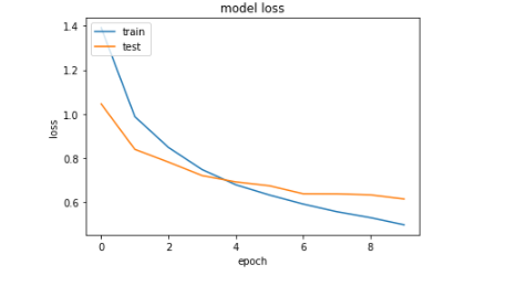
The model defined above will be trained now, where we use 0.005 as our initial learning rate and training batch size of 64. We will be training our model for 10 epochs, in which we have taken categorical cross-entropy loss as our loss function and Adamax optimizer for convergence.
We additionally define a learning rate scheduler, which decays the learning rate after each epoch.
| def lr_scheduler(epoch): | |
| return INIT_LR * 0.9 ** epoch |
We also define a class that handles callbacks from Keras. It prints out the learning rate used in that epoch.
| class LrHistory(tf.keras.callbacks.Callback): | |
| def on_epoch_begin(self, epoch, logs={}): | |
| print("Learning rate:", tf.keras.backend.get_value(model.optimizer.lr)) |
Finally, after defining and training we save our model to a disk for future evaluation!
Evaluation of our model
> Let us look at the learning curve during the training of our model.
> Let us predict the classes for each image in testing set.
| Y_pred_test = model.predict_proba(X_test_normalized) # Predict probability of image belonging to a class, for each class | |
| Y_pred_test_classes = np.argmax(Y_pred_test, axis=1) # Class with highest probability from predicted probabilities | |
| Y_test_classes = np.argmax(Y_test_coded, axis=1) # Actual class | |
| Y_pred_test_max_probas = np.max(Y_pred_test, axis=1) # Highest probability |
> Let us look at the confusion matrix to understand the performance.
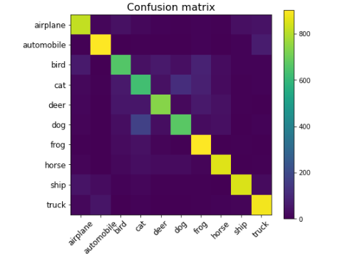
Finally the test accuracy obtained for our model is 79.11%
Compiling with deepC:
To bring the saved model on MCU, install deepC — an open-source, vendor-independent deep learning library cum compiler and inference framework, for microcomputers and micro-controllers.
| !deepCC cifar-10_model.TF --format=tensorflow |
Here’s the link to the complete notebook: https://cainvas.ai-tech.systems/use-cases/keras-cifar-10-vision-app/#
Credits: Alex krizhevsky, University of Toronto, and Vaibhav Sharma
Written by: Sanlap Dutta
Also Read: Cotton Plant Disease Detection