Deep learning to identify the species of hummingbird at your window

Of all the birds that you see every day, how many can you identify? What is that tiny bird with a long beak and a colorful neck? If it is a hummingbird, what kind? Aren’t you a little curious?
Bird watching is a task that requires experience and expertise. Here we will train neural networks to identify 3 species of hummingbirds if they are in the image.
Deep learning models trained to identify birds and their species can be used to monitor wildlife over prolonged periods of time. Human intervention, support, and input are necessary at times but this will drastically reduce the time and effort required for the task.
Implementation of the idea on cAInvas — here!
The dataset
The images in the dataset were all gathered from various hummingbird feeders in the towns of Morrison and Bailey, Colorado.
The dataset has 3 folders, train, validation, and test, each with 100, 20, and 20 images of each class label respectively.
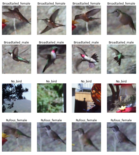
The four labels in the dataset are –
- No_bird
- Rufous_female
- Bradtailed_female
- Broadtailed_male
The image_dataset_from_directory function of the keras.preprocessing module is used to load the images into the respective datasets by passing the paths accordingly. Each sample is loaded as a 256×256 image.
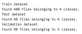
Defining the class names for use later.

A peek into a few samples from each class —
Preprocessing
Normalization
The pixel values of these images are integers in the range 0–255. Normalizing the pixel values reduces them to float values in the range [0, 1]. This is done using the Rescaling function of the keras.layers.experimental.preprocessing module.
This helps in faster convergence of the model’s loss function.
Augmentation
The dataset has only 100 images per class in the training set. This is not enough data to get good results.
Image data augmentation is a technique to artificially increase the size of the training dataset using techniques like scaling (or resizing), cropping, flipping (horizontal or vertical or both), padding, rotation, translation (movement along x or y-axis). Colour augmentation techniques include adjusting the brightness, contrast, saturation, and hue of the images.
Here, we will implement two image augmentation techniques using functions from the keras.layers.experimental.preprocessing module —
- RandomFlip — randomly flip the images along the directions specified as a parameter (horizontal or vertical or both)
- RandomZoom — random images in the dataset are zoomed 10%.
Feel free to try out other augmentation techniques!
The augmented dataset is combined with the original training set, thus doubling the number of samples available for training.
The model
We are using transfer learning, which is the concept of using the knowledge gained while solving one problem to solve another problem.
Xception architecture is an extension of the Inception architecture with depthwise separable convolutions replacing the standard Inception modules.
The model’s input is defined to have a size of (256, 256, 3).
The last layer of the Xception model (classification layer) is not included and instead, it is appended with a GlobalAveragePooling layer followed by a Dense layer with softmax activation and as many nodes as there are classes.
The model is configured such that the appended layers are the only trainable part of the entire model. This means that, as the training epochs advance, the weights of nodes in the Xception architecture remain constant.
The model is compiled using the sparse categorical cross-entropy loss function because the final layer of the model has the softmax activation function and the outputs of the model are not one-hot encoded here. The Adam optimizer is used and the accuracy of the model is tracked over epochs.
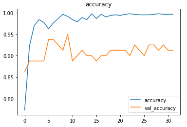
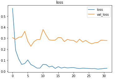
The EarlyStopping callback function of the keras.callbacks module monitors the validation loss and stops the training if it doesn’t for 3 epochs continuously. The restore_best_weights parameter ensures that the model with the least validation loss is restored to the model variable.
The model is trained first with a learning rate of 0.01 which is then reduced to 0.001.

The model achieved around 92.5% accuracy on the test set.
The metrics
Prediction
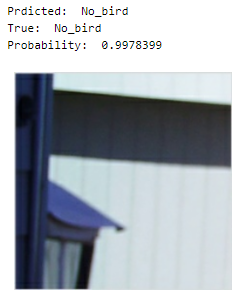
Let’s look at the test image along with the model’s prediction —
deepC
deepC library, compiler, and inference framework are designed to enable and perform deep learning neural networks by focussing on features of small form-factor devices like micro-controllers, eFPGAs, CPUs, and other embedded devices like raspberry-pi, odroid, Arduino, SparkFun Edge, RISC-V, mobile phones, x86 and arm laptops among others.
Compiling the model using deepC —

Head over to the cAInvas platform (link to notebook given earlier) to run and generate your own .exe file!
Credits: Ayisha D
Also Read: Epileptic seizure recognition — on cAInvas
