Heart Disease Prediction using Neural Networks
Photo by Diana Pasternak on Dribbble

Heart disease refers to any condition affecting the heart. There are many types, some of which are preventable. Share on Pinterest mikroman6/Getty Images. Unlike a cardiovascular disease, which includes problems with the entire circulatory system, heart disease affects only the heart.

This project will focus on predicting heart disease using neural networks. Based on attributes such as blood pressure, cholesterol levels, heart rate, and other characteristic attributes, patients will be classified according to varying degrees of coronary artery disease. This project will utilize a dataset of 303 patients and distributed by the UCI Deep Learning Repository.

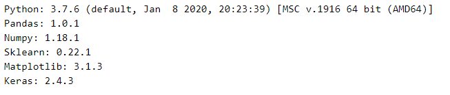
We will be using some common Python libraries, such as pandas, NumPy, and matplotlib. Furthermore, for the deep learning side of this project, we will be using sklearn and Keras.

In this project, we are going into the sequence, and follow steps one by one:


Importing necessary libraries

import sys
import pandas as pd
import numpy as np
import sklearn
import matplotlib
import keras
print('Python: {}'.format(sys.version))
print('Pandas: {}'.format(pd.__version__))
print('Numpy: {}'.format(np.__version__))
print('Sklearn: {}'.format(sklearn.__version__))
print('Matplotlib: {}'.format(matplotlib.__version__))
print('Keras: {}'.format(keras.__version__))

Importing necessary libraries

import matplotlib.pyplot as plt
from pandas.plotting import scatter_matrix
import seaborn as sns

Importing the Dataset

Now, we are importing the dataset or say we are reading the dataset.

This dataset contains patient data concerning heart disease diagnosis that was collected at several locations around the world. There are 76 attributes, including age, sex, resting blood pressure, cholesterol levels, echocardiogram data, exercise habits, and many others.

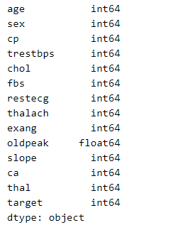
To data, all published studies using this data focus on a subset of 14 attributes — so we will do the same. More specifically, we will use the data collected at the Cleveland Clinic Foundation.

# read the csv
cleveland = pd.read_csv('heart.csv')

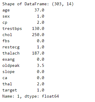
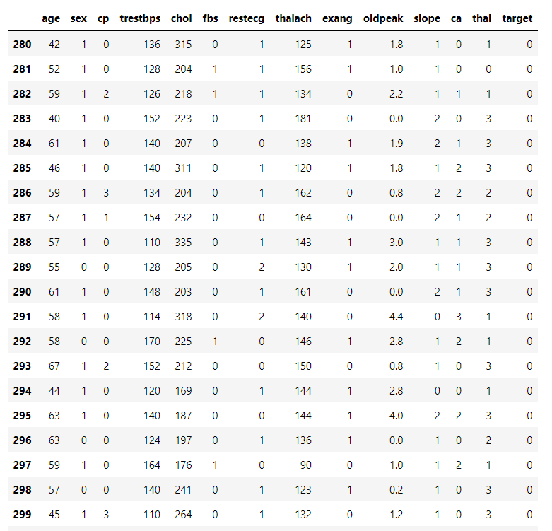
Now, we are printing the dataframe, so we can see how many examples we have.

print( 'Shape of DataFrame: {}'.format(cleveland.shape))
print (cleveland.loc[1])

Importing the Dataset

Now, for preprocessing the data, we remove missing data (indicated with a “?”).

data = cleveland[~cleveland.isin(['?'])]
data.loc[280:]

Importing the Dataset

Now, we are dropping the rows with NaN values from DataFrame.

data = data.dropna(axis=0)
data.loc[280:]

Importing the Dataset of Heart Disease Patient

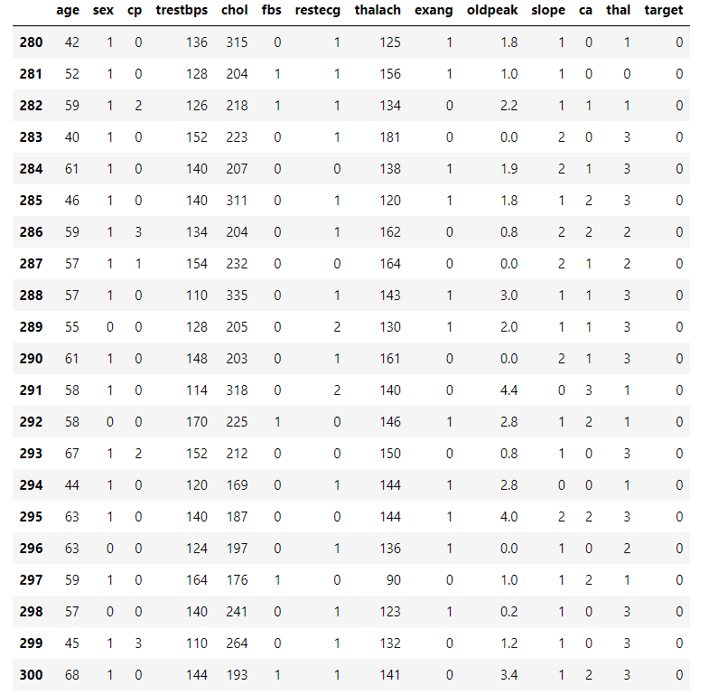
Now, we transform data to numeric to enable further analysis.

data = data.apply(pd.to_numeric)
data.dtypes

transform data to numeric

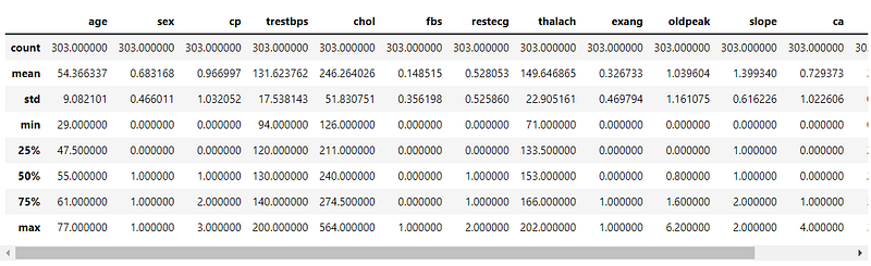
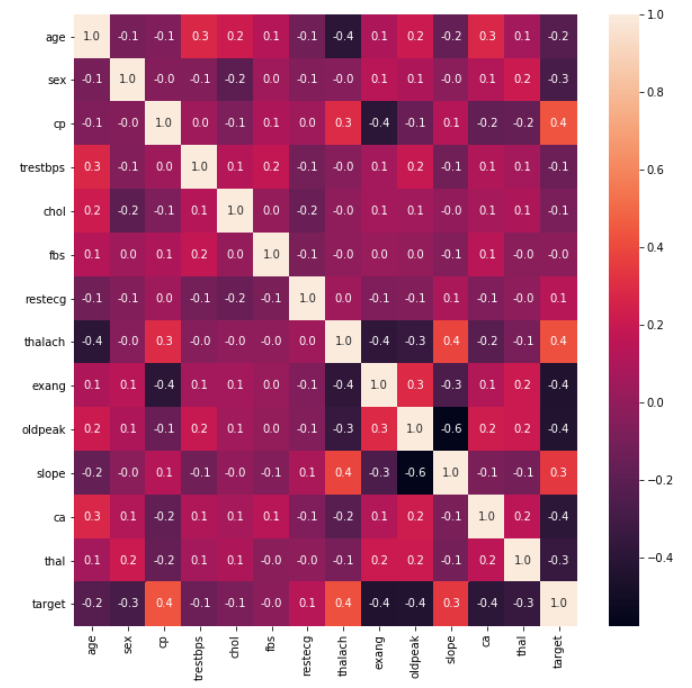
Now, we print data characteristics, using pandas built-in describe() function.

data.describe()

print data characteristics

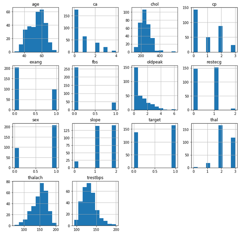
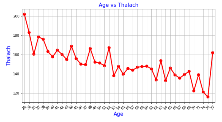
Now, we are plotting the histograms for each variable.

data.hist(figsize = (12, 12))
plt.show()

Plotting the histograms for each variable

pd.crosstab(data.age,data.target).plot(kind="bar",figsize=(20,6))
plt.title('Heart Disease Frequency for Ages')
plt.xlabel('Age')
plt.ylabel('Frequency')
plt.show()

plotting the histograms for each variable

plt.figure(figsize=(10,10))
sns.heatmap(data.corr(),annot=True,fmt='.1f')
plt.show()

plotting the histograms for each variable

age_unique=sorted(data.age.unique())
age_thalach_values=data.groupby('age')['thalach'].count().values
mean_thalach=[]
for i,age in enumerate(age_unique):
mean_thalach.append(sum(data[data['age']==age].thalach)/age_thalach_values[i])
plt.figure(figsize=(10,5))
sns.pointplot(x=age_unique,y=mean_thalach,color='red',alpha=0.8)
plt.xlabel('Age',fontsize = 15,color='blue')
plt.xticks(rotation=45)
plt.ylabel('Thalach',fontsize = 15,color='blue')
plt.title('Age vs Thalach',fontsize = 15,color='blue')
plt.grid()
plt.show()

plotting the histograms for each variable

Create Training and Testing Datasets

Now that we have preprocessed the data appropriately, we can split it into training and testing datasets. We will use Sklearn’s train_test_split() function to generate a training dataset (80 percent of the total data) and a testing dataset (20 percent of the total data).

X = np.array(data.drop(['target'], 1))
y = np.array(data['target'])
X[0]

Create Training and Testing Datasets

mean = X.mean(axis=0)
X -= mean
std = X.std(axis=0)
X /= std
X[0]

Create Training and Testing Datasets

Now, we are creating X and Y datasets for training.

from sklearn import model_selection
X_train, X_test, y_train, y_test = model_selection.train_test_split(X, y, stratify=y, random_state=42, test_size = 0.2)

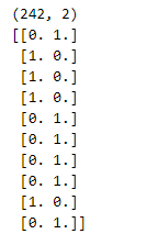
Then, we convert the data to categorical labels.

from keras.utils.np_utils import to_categorical
Y_train = to_categorical(y_train, num_classes=None)
Y_test = to_categorical(y_test, num_classes=None)
print (Y_train.shape)
print (Y_train[:10])

convert the data to categorical labels.

Building and Training the Neural Network

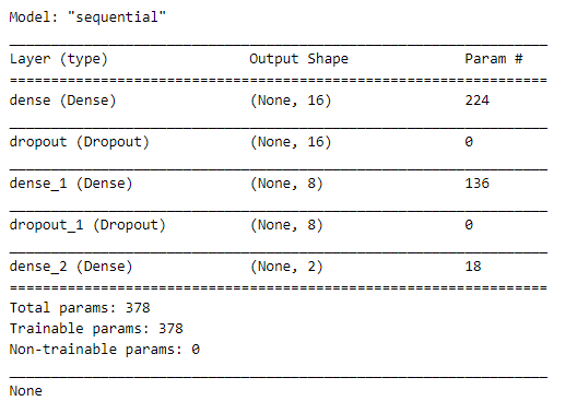
Now that we have our data fully processed and split into training and testing datasets, we can begin building a neural network to solve this classification problem. Using Keras, we will define a simple neural network with one hidden layer.

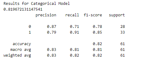
Since this is a categorical classification problem, we will use a softmax activation function in the final layer of our network and a categorical_crossentropy loss during our training phase.

from keras.models import Sequential
from keras.layers import Dense
from keras.optimizers import Adam
from keras.layers import Dropout
from keras import regularizers
# define a function to build the keras model
def create_model():
# create model
model = Sequential()
model.add(Dense(16, input_dim=13, kernel_initializer='normal', kernel_regularizer=regularizers.l2(0.001), activation='relu'))
model.add(Dropout(0.25))
model.add(Dense(8, kernel_initializer='normal', kernel_regularizer=regularizers.l2(0.001), activation='relu'))
model.add(Dropout(0.25))
model.add(Dense(2, activation='softmax'))
# compile model
adam = Adam(lr=0.001)
model.compile(loss='categorical_crossentropy', optimizer='rmsprop', metrics=['accuracy'])
return model
model = create_model()
print(model.summary())

Building and Training the Neural Network

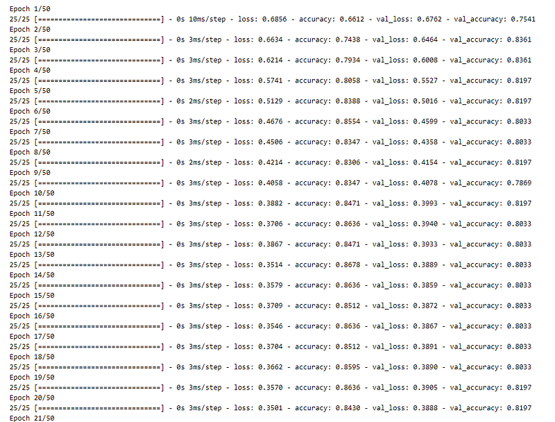
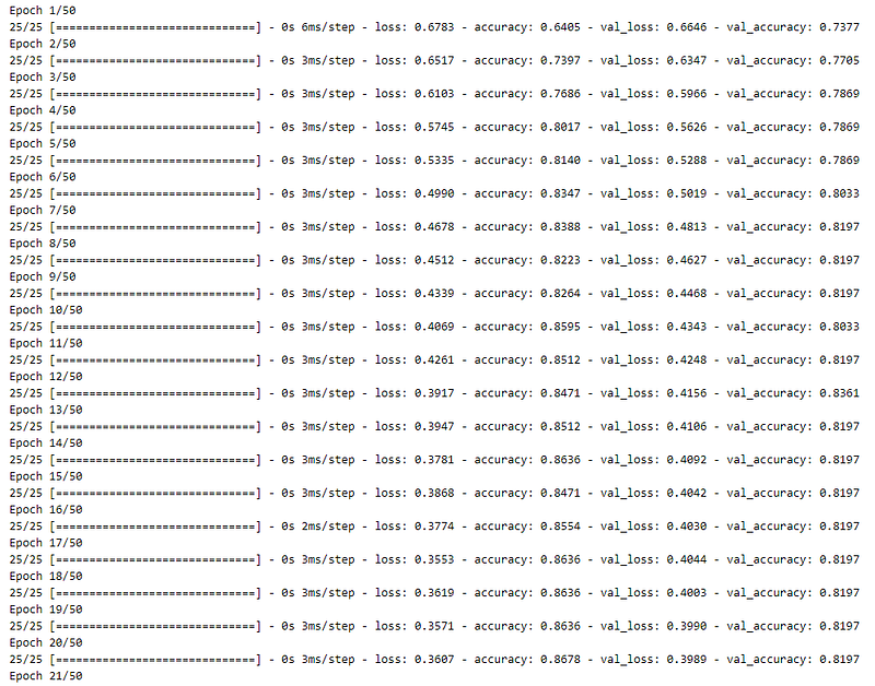
Now, we fit the model to the training data.

history=model.fit(X_train, Y_train, validation_data=(X_test, Y_test),epochs=50, batch_size=10)

fit the model to the training data

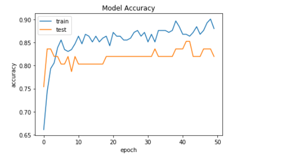
Now, we are plotting the graph of model accuracy.

import matplotlib.pyplot as plt
%matplotlib inline
# Model accuracy
plt.plot(history.history['accuracy'])
plt.plot(history.history['val_accuracy'])
plt.title('Model Accuracy')
plt.ylabel('accuracy')
plt.xlabel('epoch')
plt.legend(['train', 'test'])
plt.show()

plotting the graph of model accuracy

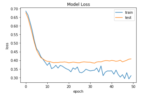
Now, we are plotting the graph of model loss.

# Model Losss
plt.plot(history.history['loss'])
plt.plot(history.history['val_loss'])
plt.title('Model Loss')
plt.ylabel('loss')
plt.xlabel('epoch')
plt.legend(['train', 'test'])
plt.show()

plotting the graph of model accuracy

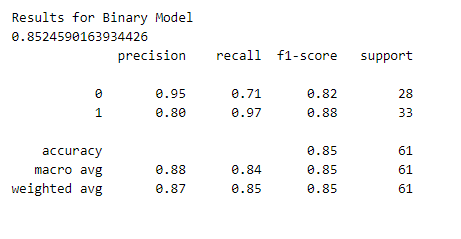
Improving Results — A Binary Classification Problem

Although we achieved promising results, we still have a fairly large error. This could be because it is very difficult to distinguish between the different severity levels of heart disease (classes 1–4). Let’s simplify the problem by converting the data to a binary classification problem — heart disease or no heart disease.

# convert into binary classification problem - heart disease or no heart disease
Y_train_binary = y_train.copy()
Y_test_binary = y_test.copy()
Y_train_binary[Y_train_binary > 0] = 1
Y_test_binary[Y_test_binary > 0] = 1
print(Y_train_binary[:20])

binary classification problem

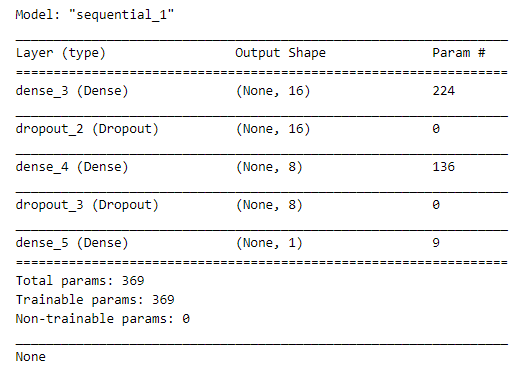
Now, we define a new Keras model for binary classification, and then later we also check the model accuracy and model loss by plotting their required graphs.

# define a new keras model for binary classification
def create_binary_model():
# create model
model = Sequential()
model.add(Dense(16, input_dim=13, kernel_initializer='normal', kernel_regularizer=regularizers.l2(0.001),activation='relu'))
model.add(Dropout(0.25))
model.add(Dense(8, kernel_initializer='normal', kernel_regularizer=regularizers.l2(0.001),activation='relu'))
model.add(Dropout(0.25))
model.add(Dense(1, activation='sigmoid'))
# Compile model
adam = Adam(lr=0.001)
model.compile(loss='binary_crossentropy', optimizer='rmsprop', metrics=['accuracy'])
return model
binary_model = create_binary_model()
print(binary_model.summary())

binary classification problem

# fit the binary model on the training data
history=binary_model.fit(X_train, Y_train_binary, validation_data=(X_test, Y_test_binary), epochs=50, batch_size=10)

Keras model for binary classification

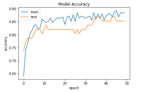
Now, we plot the graph of model accuracy but this time this is for the binary classification model.

import matplotlib.pyplot as plt
%matplotlib inline
# Model accuracy
plt.plot(history.history['accuracy'])
plt.plot(history.history['val_accuracy'])
plt.title('Model Accuracy')
plt.ylabel('accuracy')
plt.xlabel('epoch')
plt.legend(['train', 'test'])
plt.show()

plot the graph of model accuracy

Now, we plot the graph of model loss.

# Model Losss
plt.plot(history.history['loss'])
plt.plot(history.history['val_loss'])
plt.title('Model Loss')
plt.ylabel('loss')
plt.xlabel('epoch')
plt.legend(['train', 'test'])
plt.show()

plot the graph of model loss

Results and Metrics

The accuracy results we have been seeing are for the training data, but what about the testing dataset? If our models cannot generalize to data that wasn’t used to train them, they won’t provide any utility.

Let’s test the performance of both our categorical model and binary model. To do this, we will make predictions on the training dataset and calculate performance metrics using Sklearn.

# generate classification report using predictions for categorical model
from sklearn.metrics import classification_report, accuracy_score
categorical_pred = np.argmax(model.predict(X_test), axis=1)
print('Results for Categorical Model')
print(accuracy_score(y_test, categorical_pred))
print(classification_report(y_test, categorical_pred))

calculate performance metrics using Sklearn

# generate classification report using predictions for binary model
from sklearn.metrics import classification_report, accuracy_score
# generate classification report using predictions for binary model
binary_pred = np.round(binary_model.predict(X_test)).astype(int)
print('Results for Binary Model')
print(accuracy_score(Y_test_binary, binary_pred))
print(classification_report(Y_test_binary, binary_pred))

Also Read: Brain Tumor Detection

Now, we save our model

model.save('heart_disease.h5')

This is all about the heart disease prediction project.

You can download or go through the notebook from the link given here.

Credit: Bhupendra Singh Rathore

You may also be interested in 

Become a Contributor: Write for AITS Publication Today! We’ll be happy to publish your latest article on data science, artificial intelligence, machine learning, deep learning, and other technology topics.