Classification on Organic Compounds

Built a simple Artificial Neural Network using TensorFlow and Keras which classifies the organic compounds as either Musk or Non-Musk compounds

Aim

To develop a Deep Learning model that classifies the organic compounds as either Musk or Non-Musk compounds using python programming language and Deep learning libraries

Prerequisites

Before getting started, you should have a good understanding of:

Python programming language
Deep Learning Libraries(Tensorflow, Keras)

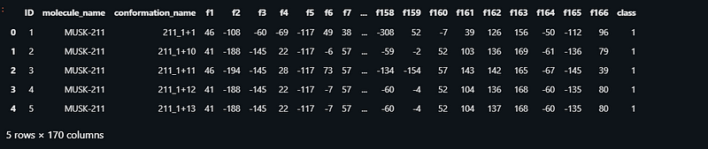
Dataset

Link to download the dataset:

https://datahub.io/machine-learning/musk

get the data

	# get data file
	!wget -N "https://cainvas-static.s3.amazonaws.com/media/user_data/vomchaithany/musk.csv"

view raw gistfile1.txt hosted with ❤ by GitHub

output:

--2021-07-06 11:17:20--  https://cainvas-static.s3.amazonaws.com/media/user_data/vomchaithany/musk.csv
Resolving cainvas-static.s3.amazonaws.com (cainvas-static.s3.amazonaws.com)... 52.219.160.35
Connecting to cainvas-static.s3.amazonaws.com (cainvas-static.s3.amazonaws.com)|52.219.160.35|:443... connected.
HTTP request sent, awaiting response... 304 Not Modified
File ‘musk.csv’ not modified on server. Omitting download.

Import the required libraries

	# Import the required libraries
	import tensorflow as tf
	import pandas as pd
	import matplotlib.pyplot as plt

view raw gistfile1.txt hosted with ❤ by GitHub

Load the data

	# read the csv file
	dataset = pd.read_csv('musk.csv')
	dataset.head()

view raw gistfile1.txt hosted with ❤ by GitHub

output:

Preprocessing the Data

	X = dataset.iloc[:, 3:-1].values
	y = dataset.iloc[:, -1].values

	# Scaling
	from sklearn.preprocessing import StandardScaler
	ss = StandardScaler()
	X = ss.fit_transform(X)

view raw gistfile1.txt hosted with ❤ by GitHub

Split the data for training and test

	from sklearn.model_selection import train_test_split
	X_train, X_test, y_train, y_test = train_test_split(X, y, test_size = 0.3, random_state = 42)

	X_train.shape,y_train.shape

view raw gistfile1.txt hosted with ❤ by GitHub

output:

((4618, 166), (4618,))

Build, train, and save the model

	model = tf.keras.models.Sequential([
	tf.keras.layers.Dense(33, input_shape=(166,),
	activation=tf.nn.tanh),
	tf.keras.layers.Dense(1, activation=tf.nn.sigmoid)
	])

	# compile
	model.compile(optimizer='adam', loss='binary_crossentropy', metrics=['accuracy'])

	history = model.fit(X_train, y_train, validation_data = (X_test, y_test), epochs = 15)

	# Save the model
	model.save("Simple ANN.h5")

view raw gistfile1.txt hosted with ❤ by GitHub

output:

Epoch 1/15
145/145 [==============================] - 0s 3ms/step - loss: 0.4019 - accuracy: 0.8441 - val_loss: 0.2712 - val_accuracy: 0.9157
Epoch 2/15
145/145 [==============================] - 0s 2ms/step - loss: 0.2232 - accuracy: 0.9309 - val_loss: 0.1938 - val_accuracy: 0.9444
Epoch 3/15
145/145 [==============================] - 0s 2ms/step - loss: 0.1743 - accuracy: 0.9461 - val_loss: 0.1602 - val_accuracy: 0.9480
Epoch 4/15
145/145 [==============================] - 0s 2ms/step - loss: 0.1454 - accuracy: 0.9530 - val_loss: 0.1333 - val_accuracy: 0.9601
Epoch 5/15
145/145 [==============================] - 0s 2ms/step - loss: 0.1238 - accuracy: 0.9591 - val_loss: 0.1167 - val_accuracy: 0.9641
Epoch 6/15
145/145 [==============================] - 0s 2ms/step - loss: 0.1095 - accuracy: 0.9632 - val_loss: 0.1033 - val_accuracy: 0.9682
Epoch 7/15
145/145 [==============================] - 0s 2ms/step - loss: 0.0946 - accuracy: 0.9693 - val_loss: 0.0946 - val_accuracy: 0.9646
Epoch 8/15
145/145 [==============================] - 0s 2ms/step - loss: 0.0848 - accuracy: 0.9725 - val_loss: 0.0859 - val_accuracy: 0.9717
Epoch 9/15
145/145 [==============================] - 0s 2ms/step - loss: 0.0758 - accuracy: 0.9766 - val_loss: 0.0798 - val_accuracy: 0.9732
Epoch 10/15
145/145 [==============================] - 0s 2ms/step - loss: 0.0700 - accuracy: 0.9783 - val_loss: 0.0737 - val_accuracy: 0.9737
Epoch 11/15
145/145 [==============================] - 0s 2ms/step - loss: 0.0611 - accuracy: 0.9831 - val_loss: 0.0670 - val_accuracy: 0.9783
Epoch 12/15
145/145 [==============================] - 0s 2ms/step - loss: 0.0548 - accuracy: 0.9842 - val_loss: 0.0622 - val_accuracy: 0.9803
Epoch 13/15
145/145 [==============================] - 0s 2ms/step - loss: 0.0505 - accuracy: 0.9857 - val_loss: 0.0612 - val_accuracy: 0.9798
Epoch 14/15
145/145 [==============================] - 0s 2ms/step - loss: 0.0452 - accuracy: 0.9861 - val_loss: 0.0564 - val_accuracy: 0.9823
Epoch 15/15
145/145 [==============================] - 0s 2ms/step - loss: 0.0404 - accuracy: 0.9883 - val_loss: 0.0546 - val_accuracy: 0.9828

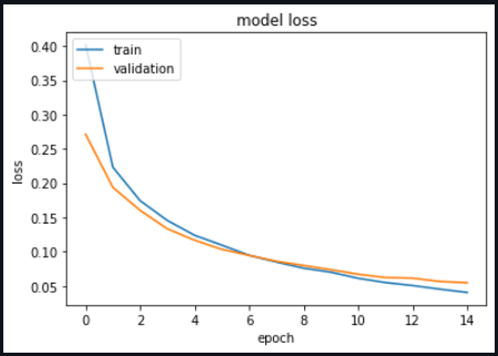
Graphs

loss vs validation loss

	from matplotlib import pyplot as plt
	plt.plot(history.history['loss'])
	plt.plot(history.history['val_loss'])
	plt.title('model loss')
	plt.ylabel('loss')
	plt.xlabel('epoch')
	plt.legend(['train', 'validation'], loc='upper left')
	plt.show()

view raw gistfile1.txt hosted with ❤ by GitHub

output:

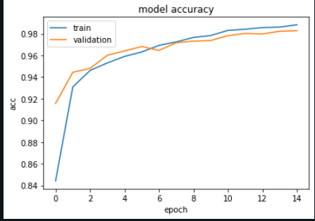
Accuracy vs validation accuracy

	from matplotlib import pyplot as plt
	plt.plot(history.history['accuracy'])
	plt.plot(history.history['val_accuracy'])
	plt.title('model accuracy')
	plt.ylabel('acc')
	plt.xlabel('epoch')
	plt.legend(['train', 'validation'], loc='upper left')
	plt.show()

view raw gistfile1.txt hosted with ❤ by GitHub

output:

Accuracy of our model

	# accuracy and loss
	model.evaluate(X_test, y_test)

view raw gistfile1.txt hosted with ❤ by GitHub

output:

62/62 [==============================] - 0s 1ms/step - loss: 0.0546 - accuracy: 0.9828
[0.0546199269592762, 0.9828282594680786]

Predictions

	y_pred = model.predict(X_test)
	y_pred[5:10]

view raw gistfile1.txt hosted with ❤ by GitHub

output:

array([[1.4935225e-03],
       [6.3299501e-01],
       [3.2852648e-03],
       [7.9143688e-04],
       [2.2959751e-04]], dtype=float32)

	y_pred1 = []
	for element in y_pred:
	if element > 0.5:
	y_pred1.append(1)
	else:
	y_pred1.append(0)

	y_pred1[25:40]

view raw gistfile1.txt hosted with ❤ by GitHub

output:

[0, 0, 0, 0, 0, 0, 0, 0, 0, 0, 1, 0, 0, 0, 0]

y_test[25:40]

view raw gistfile1.txt hosted with ❤ by GitHub

output:

array([0, 0, 0, 0, 0, 0, 0, 0, 0, 0, 1, 0, 0, 0, 0])

here we can see that the predicted values are the same as the actual values

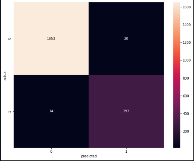
Classification report and Heat Map

	# print the classification report
	from sklearn.metrics import classification_report, confusion_matrix
	print(classification_report(y_test,y_pred1))

view raw gistfile1.txt hosted with ❤ by GitHub

output

precision    recall  f1-score   support

           0       0.99      0.99      0.99      1673
           1       0.94      0.95      0.95       307

    accuracy                           0.98      1980
   macro avg       0.96      0.97      0.97      1980
weighted avg       0.98      0.98      0.98      1980

Heat Map

	import seaborn as sn

	cm = tf.math.confusion_matrix(labels = y_test, predictions = y_pred1)

	plt.figure(figsize = (10,8))
	sn.heatmap(cm, annot = True, fmt = 'd')
	plt.xlabel("predicted")
	plt.ylabel("actual")

view raw gistfile1.txt hosted with ❤ by GitHub

output:

Link to access the notebook:

Conclusion:

We’ve trained our simple ANN using TensorFlow and Keras for classifying Musk /Non-Musk compounds and got an accuracy of 98%.

Notebook Link: Here

Credit: Om Chaithanya V

Also Read: Detecting Ships from Aerial Imagery using Deep Learning

replica rolex milgauss

Aim

Prerequisites

Dataset

Import the required libraries

Load the data

Preprocessing the Data

Split the data for training and test

Build, train, and save the model

Graphs

Accuracy of our model

Predictions

Classification report and Heat Map

Heat Map

Conclusion:

105 Serra Way, 251, Milpitas, CA.