Tyre Pressure Detection using CNN

November 20, 2022

This Model uses Images of car’s tyre to predict whether the tyre is Full or Flat or if no tyre is detected.

The Dataset contains 3 classes — :

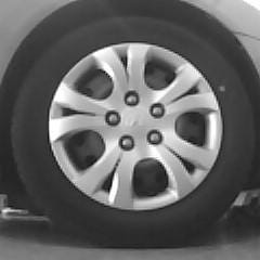
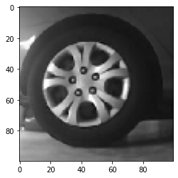
1. Full Tyre

It contains Images of car Tyres who have proper air pressure and hence they are considered full. Here is an example of how a full tyre looks -:

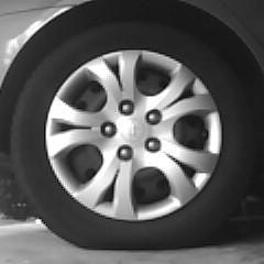
Tyre Pressure Detection using CNN: Full Tyre — Full Tyre

2. Flat Tyre

These tyres don’t have enough air pressure so they are flat i.e. they need to be filled again and checked or else it may become the very reason of an accident. Here is an example of how a flat tyre looks -:

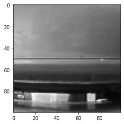
Tyre Pressure Detection using CNN: Flat Tyre — Flat Tyre

3. No- Tyre

These images represent the scenario when the image contains something else other than a tyre or it may not contain proper image of tyre. Here is an example of no- tyre class :-

Tyre Pressure Detection using CNN: No-Tyre — No-Tyre

Here is a demonstration of how to build this model using Tensorflow and Keras using Python.

Importing Libraries

	import numpy as np
	import pandas as pd
	import seaborn as sns
	import matplotlib.pyplot as plt
	from sklearn.preprocessing import StandardScaler
	from sklearn.model_selection import train_test_split
	import tensorflow as tf
	import cv2 as cv
	from sklearn import preprocessing
	from tensorflow import keras
	from tensorflow.keras.layers import Conv2D, MaxPooling2D, Flatten, Dropout, Dense
	from tensorflow.keras import layers
	from tensorflow.keras.models import Sequential
	from tensorflow.keras.preprocessing.image import load_img, img_to_array
	from tensorflow.keras.layers import Dense, Dropout, Activation
	from tensorflow.keras.callbacks import ModelCheckpoint

view raw importing libraries.py hosted with ❤ by GitHub

Loading the Dataset

	!wget "https://cainvas-static.s3.amazonaws.com/media/user_data/tanmay/tyre.zip"
	!unzip -qo tyre.zip

view raw loading dataset.py hosted with ❤ by GitHub

Preprocessing

	train_dir= "./tire-dataset/"
	train_datagen= tf.keras.preprocessing.image.ImageDataGenerator(rescale= 1./255, validation_split=0.2)
	train_generator= train_datagen.flow_from_directory(train_dir, target_size= (100,100), color_mode= 'grayscale', batch_size= 20, class_mode= 'categorical', subset= 'training')
	val_generator= train_datagen.flow_from_directory(train_dir, target_size= (100,100), color_mode= 'grayscale', batch_size= 20, class_mode= 'categorical', subset= 'validation')

view raw preprocessing.py hosted with ❤ by GitHub

Model Building

	model= Sequential([
	layers.Conv2D(32, (3,3), activation= 'relu', input_shape= (100,100,1)),
	layers.MaxPooling2D(pool_size= (2,2), padding= 'same'),
	layers.Dropout(0.3),
	layers.Conv2D(16, (3,3), activation= 'relu'),
	layers.MaxPooling2D(pool_size= (2,2), padding= 'same'),
	layers.Flatten(),
	layers.Dropout(0.3),
	layers.Dense(25, activation= 'relu'),
	# layers.Dense(64, activation= 'relu'),
	layers.Dense(3, activation= 'softmax')
	])
	model.compile(optimizer= 'adam', loss= 'categorical_crossentropy', metrics= ['accuracy'])

view raw build.py hosted with ❤ by GitHub

Model Fitting

history= model.fit_generator(train_generator, epochs= 20, validation_data= val_generator)

view raw fit.py hosted with ❤ by GitHub

Plotting Accuracy of Model

	plt.plot(history.history['accuracy'])
	plt.plot(history.history['val_accuracy'])
	plt.title("Model Accuracy")
	plt.xlabel("Epoch")
	plt.ylabel("Accuracy")
	plt.legend(["Train", "Test"], loc= "lower right");

view raw pltacc.py hosted with ❤ by GitHub

Plotting Loss of Model

	plt.plot(history.history['loss'])
	plt.plot(history.history['val_loss'])
	plt.title('Model Loss')
	plt.xlabel('Epoch')
	plt.ylabel('Loss')
	plt.legend(['Train','Test'], loc= 'upper right');

view raw pltloss.py hosted with ❤ by GitHub

Predictions

	tyre = ["Flat Tyre","Full Tyre","No Tyre"]
	def Single_Image_Prediction(file):
	#image = load_img(file, color_mode='rgb', target_size=(128, 128))
	image= file
	plt.imshow(image,cmap= 'gray')
	plt.show()
	print(image.shape)
	# cv.imshow('image',file)
	# cv.waitKey(0)
	# cv.destroyAllWimdows()
	# image = cv.cvtColor(image, cv.COLOR_RGB2GRAY)
	img_arr = img_to_array(image)
	# img_arr = img_arr/255.
	np_image = np.expand_dims(img_arr, axis=0)
	return np_image

	image = Single_Image_Prediction(val_generator[0][0][11])
	pred_value = model.predict(image)
	print(pred_value)
	index_value = np.argmax(pred_value,axis=1) #For categorical model
	print(tyre[index_value[0]])

	image = Single_Image_Prediction(val_generator[0][0][12])
	pred_value = model.predict(image)
	print(pred_value)
	index_value = np.argmax(pred_value,axis=1) #For categorical model
	print(tyre[index_value[0]])

	image = Single_Image_Prediction(val_generator[0][0][0])
	pred_value = model.predict(image)
	print(pred_value)
	index_value = np.argmax(pred_value,axis=1) #For categorical model
	print(tyre[index_value[0]])

view raw predictions.py hosted with ❤ by GitHub

We can see that our Model is performing well which the Predictions are verifying also. Now we will save our Model.

Saving and deepCC

deepCC is a framework which converts the Deep Learning Models into an executable file which can be used in IOT devices like Arduino, MCU’s, etc.

	model.save('tyre_v1.h5')
	!deepCC tyre_v1.h5

view raw saving.py hosted with ❤ by GitHub

Here is the link for the Notebook — Click Here

Thank you for reading this article, have a great day!

Credit: Tanmay Mishra